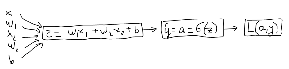
Logistic Regression:
\(z = w^T x + b\)
\(\hat{y} = a = \sigma(z)\)
\(L(a, y) = -(ylog(a) + (1-y)log(1-a))\)
Then, computation graph is:
 \(\frac{\partial L}{\partial a} = -\frac{y}{a} + \frac{1-y}{1-a}\) and \(\frac{\partial a}{\partial z} = a(1-a) \) (derivative of sigmoid function)
then, \(\frac{\partial L}{\partial z} = \frac{\partial L}{\partial a} * \frac{\partial a}{\partial z} = a-y\)
Finally,
\(\frac{\partial L}{\partial w_1} = \frac{\partial L}{\partial z} * \frac{\partial z}{\partial w_1} = (a-y) * x_1 \), \(\frac{\partial L}{\partial x_1} = \frac{\partial L}{\partial z} * \frac{\partial z}{\partial x_1} = (a-y) * w_1 \)
\(\frac{\partial L}{\partial w_2} = \frac{\partial L}{\partial z} * \frac{\partial z}{\partial w_2} = (a-y) * x_2 \), \(\frac{\partial L}{\partial x_2} = \frac{\partial L}{\partial z} * \frac{\partial z}{\partial x_1} = (a-y) * w_2 \)
\(\frac{\partial L}{\partial b} = \frac{\partial L}{\partial z} * \frac{\partial z}{\partial b} = (a-y) * 1 = (a-y) \)
From here, we can use Gradient Descent algorithm to update w and b
Algorithm for m training examples: (suppose n_x = 2)
for i from 1 to m: {
}
Then \(J {/}{=} m, d w_1 {/}{=} m, d w_2 {/}{=} m, d b {/}{=} m\)
Then run repeat simultaneous update for \(w_1, w_2, b \) until converges
Vectorization: get rid of for loops taking advantage of parallelism
z = np.dot(w, x)
Rule of thumbs: whenever possible, avoid explicit for-loops
u = Av => u = np.dot(A, v)
v, find u = exp(v) => u = np.exp(v)
Above algorithm in vectorized form in python using numpy:
\(Z = np.dot(w.T, X) + b\) (b is made into an (1 x m) row vector by python's broadcasting
\(A = \sigma(Z)\)
\(dZ = A - Y\)
\(dw = \frac{1}{m} X dZ^T\)
\(db = \frac{1}{m} np.sum(dZ)\)
Where
\( X \in R^{n_x \times m} \\
b, Y, Z, A \in R^{1 \times m} \\
w, dw \in R^{n_x \times 1} \\
b \in R \)
Then run repeat simultaneous update \(w := w - \alpha dw, b := b - \alpha db\)
We still need a for (or while) loop over multiple iterations of gradient descent
\(z = w^T x + b\)
\(\hat{y} = a = \sigma(z)\)
\(L(a, y) = -(ylog(a) + (1-y)log(1-a))\)
Then, computation graph is:
then, \(\frac{\partial L}{\partial z} = \frac{\partial L}{\partial a} * \frac{\partial a}{\partial z} = a-y\)
Finally,
\(\frac{\partial L}{\partial w_1} = \frac{\partial L}{\partial z} * \frac{\partial z}{\partial w_1} = (a-y) * x_1 \), \(\frac{\partial L}{\partial x_1} = \frac{\partial L}{\partial z} * \frac{\partial z}{\partial x_1} = (a-y) * w_1 \)
\(\frac{\partial L}{\partial w_2} = \frac{\partial L}{\partial z} * \frac{\partial z}{\partial w_2} = (a-y) * x_2 \), \(\frac{\partial L}{\partial x_2} = \frac{\partial L}{\partial z} * \frac{\partial z}{\partial x_1} = (a-y) * w_2 \)
\(\frac{\partial L}{\partial b} = \frac{\partial L}{\partial z} * \frac{\partial z}{\partial b} = (a-y) * 1 = (a-y) \)
From here, we can use Gradient Descent algorithm to update w and b
Algorithm for m training examples: (suppose n_x = 2)
for i from 1 to m: {
- \(z^{(i)} = w^T x^{(i)} + b \)
- \(a^{(i)} = \hat{y}^{(i)} = \sigma (z^{(i)}) \)
- \(d z^{(i)} = a^{(i)} - y^{(i)} \)
- \(J {+}{=} - (y^{(i)}log(a^{(i)}) + (1-y)^{(i)}log(1 - a^{(i)})) \)
- \(d w_1 {+}{=} x_{1}^{(i)} d z^{(i)} \)
- \(d w_2 {+}{=} x_{2}^{(i)} d z^{(i)} \)
- \(d b {+}{=} d z^{(i)} \)
}
Then \(J {/}{=} m, d w_1 {/}{=} m, d w_2 {/}{=} m, d b {/}{=} m\)
Then run repeat simultaneous update for \(w_1, w_2, b \) until converges
Vectorization: get rid of for loops taking advantage of parallelism
z = np.dot(w, x)
Rule of thumbs: whenever possible, avoid explicit for-loops
u = Av => u = np.dot(A, v)
v, find u = exp(v) => u = np.exp(v)
Above algorithm in vectorized form in python using numpy:
\(Z = np.dot(w.T, X) + b\) (b is made into an (1 x m) row vector by python's broadcasting
\(A = \sigma(Z)\)
\(dZ = A - Y\)
\(dw = \frac{1}{m} X dZ^T\)
\(db = \frac{1}{m} np.sum(dZ)\)
Where
\( X \in R^{n_x \times m} \\
b, Y, Z, A \in R^{1 \times m} \\
w, dw \in R^{n_x \times 1} \\
b \in R \)
Then run repeat simultaneous update \(w := w - \alpha dw, b := b - \alpha db\)
We still need a for (or while) loop over multiple iterations of gradient descent
Comments
Post a Comment